Statistics assignment: Analysis on Social Progress Index of 2019

Question

Task: Most of your statistical calculations should be carried out using Excel only and you will use Microsoft Word and Excel to complete this assignment.

1. Select a Random Sample
Select a random sample of size 100 from the given 182 countries (as demonstrated in videos of e-tivity 1.1). Remember that 182 countries constitute the population of interest and do not calculate any parameters such as mean and standard deviation from the population. Then from each category with an even number (categories 2, 4, 6, 8, 10 and 12), select one variable only. For example, under category 2, Water and Sanitation, there are three variables. They are:

• Access to piped water
• Rural access to improved water source
• Access to improved sanitation facilities

Answer

Introduction
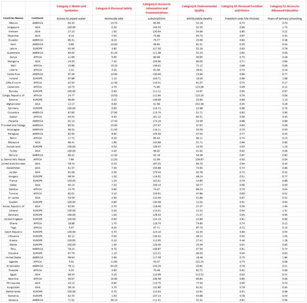
The given report on statistics assignment aims to highlight the appropriate responses for the questions posed by Margaret based on the results obtained by conducting the statistical analysis on the sample data set of Social Progress Index of 2019. Also, the various comparisons among the countries has been drawn at each of the sub categories highlighted in the index so as to find the importance of Social Progress Index.The sample size has been taken a 100 but after removing the missing values row from the data the sample has been reduced to 66. The sample data and the statistical analysis have been shown in the Appendix highlighted at the end of the statistics assignment.

Analysis
Descriptive Statistics

1) Continent

It can be seen from the above analysis presented in the statistics assignment that maximum percentages of countries included in the sample belong to Europe. Also, the lowest representation of the countries is from America which has a representation of 23% in the total sample data. The above representation indicates that the four major continents have a fair representation in the underlying sample.

2) Access to piped water

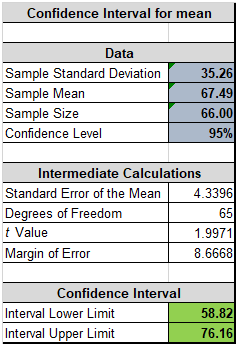
The average access to piped water is found as 67.49 but it is quite influenced through the presence of the outliers present in the higher side. Therefore, it is stated herein statistics assignment that the median would be termed as suitable measure of central tendency whereas, the inter quartile range is the appropriate measure for the dispersion. The lower mean value implies that there are some countries included in the sample which have abnormally low access to piped water which is not surprising (Hair et. al., 2015).

3) Homicide rate

For while most countries, the homicide rates are low but there are certain countries for which it is quite high indicating that in such countries there is high prevalence of violence and law & order situation is questionable.

4) Mobile telephone subscriptions

It is evident from the above data shown in the statistics assignment that the mean and median of the mobile telephone subscription does not show any significant difference in the magnitude. It also implies that the distribution of the data set does not show any skew. Also, the amount of variation is quite high based on the coefficient of variation and Inter Quartile Range (Hillier, 2016).
5) Outdoor air pollution attributable deaths

The mean value of outdoor air pollution attributable deaths comes out to be 54.63 which is more than the median value. It shows that the data is skewed towards the right which is apparent from the long tail of the graph. The outdoor air pollution attributable deaths are quite high in some countries highlighting the intensity of this problem.
6) Freedom over life choices

The mean and median score obtained from the analysis done in the statistics assignment is almost the same which indicates that skew is almost absent. Also, the interquartile range indicates at dispersion in this variable being low to moderate.
7) Years of tertiary schooling

On expected lines, there seems to be high variation in the mean years of tertiary schooling. It would be expected that countries having high per capita income would have higher tertiary schooling on an average as compared to the poorer third world countries. The high range clearly indicates this disparity in the given variable (Flick, 2015).

• Confidence interval
We are 95% confident that the mean Access to Piped Water for all countries of the world would fall within the range of 58.82 and 76.16. However, there is 5% probability that the average access to piped water does not fall in the above indicated range (Hair et. al, 2015). This clearly indicates that accessibility to a basic amenity such as piped water remains a challenge in some of the poorer countries.

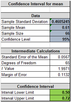
We are 95% confident that the mean year of tertiary schooling for all countries of the world would fall within the range of 0.50 and 0.72. However, there is 5% probability that the average year of tertiary schoolingdoes not fall in the above indicated range (Hillier, 2016). This clearly is indicative of the average tertiary schooling duration being quite low on a global scale.

• Hypothesis testing
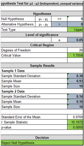
(i) Two sample hypothesis testing has been performed on variable Access to Advanced Education categories’ variable Years of tertiary schooling for Europe and Africa. The respective hypothesis testing is a right tailed test with the t stat. The computed t stats come out to be 10.1072 and the associated p value is 0.00. Assuming a significance level of 0.05. It can be concluded that mean years of tertiary schooling is more for Europe as compared to Africa.

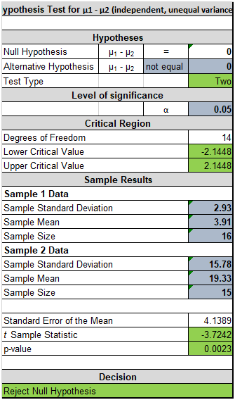
(ii) Two sample hypothesis testing has been performed on variable Homicide rate for Asian and America country. The respective hypothesis testing is a two tailed test with t stat. The computed t stats come out to be -3.7242 and the associated p value is 0.0023. Assuming a significance level of 0.05. It can be concluded that there is statistically significant difference is present in the homicide rate of Asian and American countries

(iii) Two sample hypothesis testing has been performed on Outdoor air pollution attributable deaths for Europe and America. The respective hypothesis testing is a two tailed test with the t stat. The computed t stats come out to be -1.6796 and the associated p value is 0.1038. Assuming a significance level of 0.05. It can be concluded herein statistics assignment that mean Outdoor air pollution attributable deaths for Europe and America are not different.

• Correlation and regression
(1) The relevant scatter plot has been highlighted as follows.

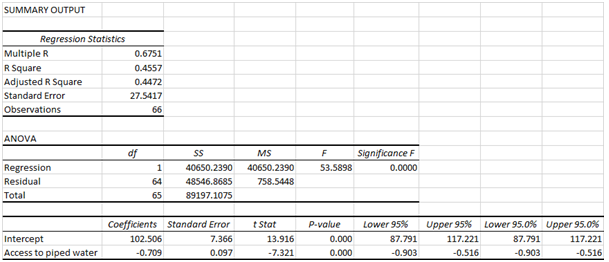
The scatterplot shown in the above context of statistics assignment highlights that their is a negative relationship exists between piped water access and attributable deaths to outdoor air pollution. Barring a couple of outliers in the given data, most of the countries seem to be situated in the vicinity of the best fit line which is indicative of the moderate to strong linear association between the given variables (Eriksson and Kovalainen, 2015). Based on the regression output attached in Appendix section of statistics assignment, the R2 value is 0.4557 which implies that 45.57% variation in the dependent variable (i.e. deaths attributed to outdoor air pollution) can be accounted for by corresponding changes in the access to piped water. Also, the p value associated with the slope is 0.00 which implies that the slope coefficient is statistically significant. A unit increase in the access to piped water would bring down the deaths attributed to outdoor air pollution by 0.709 units. Considering that the slope is significant, the regression model on the whole is also statistically significant (Flick, 2015).

(2) The relevant scatter plot has been highlighted as follows.

Considering the upward slope of the trendline, it can be concluded that a positive relationship exists between the two variables. Taking into consideration, the distribution of the scatter points about the best fit line, the strength of this relationship seems moderate (Hillier, 2014).

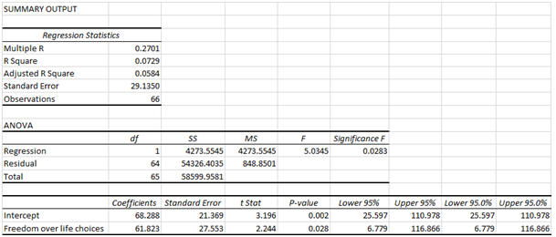
Based on the regression output attached in Appendix section of statistics assignment, the R2 value is 0.0729 which implies that 7.29% variation in the dependent variable (i.e. freedom over the life choices) can be accounted for by corresponding changes in the mobile telephone subscription. Also, the p value associated with the slope is 0.02 which implies that the slope coefficient is statistically significant at 5% significance level. A unit increase in the mobile telephone subscription would improve the freedom over life choices by 61.823 units. Considering that the slope is significant, the regression model on the whole is also statistically significant (Medhi, 2016).

Conclusion
On the basis of the statistical analysis conducted above within this statistics assignment, it can be concluded that mean Access to Piped Water for all countries lies between 58.82 and 76.16. Also, it can be concluded thatmean year of tertiary schooling for all countries would lie between 0.50 and 0.72. Further, the mean years of tertiary schooling are more for Europe as compared to Africa. Besides, the homicide rate tends to significantly vary between Asian and American countries. The average deaths attributable to outdoor air pollution do not differ between European and American countries.

A key limitation with regards to the analysis given in the statistics assignment that simple random sampling was used for the selection of countries to be included in the sample. A more appropriate choice would have been stratified random sampling considering the differences in economic and social status between various nations. Besides, from the 100 samples selected, 34 countries were removed owing to missing value which further creates a bias of under-representation and over-representation of certain attributes. Also, the results obtained within this statistics assignment must be viewed in the backdrop of the cultural and social practices that are prevalent in these countries which tend to have a profound impact. Thus, as a researcher, it is essential not to be judgmental towards the performance of different countries based on personal values and beliefs.

Appendices
Appendix 1:
Sample size

Appendix 2:
Confidence interval
1) Access to piped water

Formula
Upper Limit: Sample Mean + Margin of Error
Lower Limit: Sample Mean - Margin of Error
Margin of Error = (t value) * (Standard error)

Appendix 3:
(i) Years of Tertiary Schooling

(ii) Homicide rate

(iii) Outdoor air pollution attributable deaths

Appendix 4: Correlation and Regression
(i) Correlation matrix

Regression

(ii) Correlation matrix

Regression

References
Eriksson, P. and Kovalainen, A. (2015) Quantitative methods in business research. 3rd ed. London: Sage Publications.

Flick, U. (2015) Introducing research methodology: A beginner's guide to doing a research project. 4th ed. New York: Sage Publications.

Hair, J. F., Wolfinbarger, M., Money, A. H., Samouel, P., and Page, M. J. (2015) Essentials of business research methods.Statistics assignment2nd ed. New York: Routledge.

Hillier, F. (2016) Introduction to Operations Research.6th ed.New York: McGraw Hill Publications.

Medhi, J. (2016) Statistical Methods: An Introductory Text. 4th ed. Sydney: New Age International.