Data Analytics Assignment: Risk Analytics model for ABC Insurance Company
Question
Task
ABC Insurance Company
As of 2016, there were over 268 million registered vehicles on the roads in the United States. In 2015, there were 32,166 fatalities, 1,715,000 injuries and 4,548,000 car crashes which involved property damage. So, while many of us feel secure in our vehicles, the statistics indicate the importance of automobile insurance and in most cases, auto insurance is required by law. Auto insurance is important because it not only covers any physical damage that may occur in an accident, but also any damage or injury that might be caused because of a vehicular accident or which may be done upon oneself or one’s vehicle by another vehicle or accident – a falling tree for example(Car insurance in the U.S. - Statistics & Facts)
The Insurance industry is immensely data intensive. Historically, their data has been largely fragmented and underutilized. Also, insurance industry goes through a lot of combining structured and unstructured data, which enables the industry to generate powerful insights. With an incredible amount of data flowing in from multiple new digital channels, the insurance industry is undergoing a paradigm shift in the way they function – right from product planning to pricing, introduction, marketing, customer self-service and claim processing.
The objective of this project is to build a “Risk Analytics model” to understand the renewal potential and claim propensity of Existing Customers under Personal Auto Insurance Lines.
The question to be answered in this data analytics assignment is:
Will the policy holder initiate a claim (Yes/No) for this policy in the next policy year?
Data dictionary:
|
Sr No |
Serial Number |
|
ClaimStatus |
Indicates whether the policy holder has made a claim or not. 1 indicates a claim and 0 indicates no claim |
|
ClaimFrequency |
Gives the number of claims claimed |
|
Premium |
Premium in $1000 |
|
Billing_Term |
How often the premium is paid, i.e. once a year = 1, Three times in a year = 3, or 6 times in a year = 6 |
|
Renewed |
Indicates whether the policy has been renewed or not. 1= Renewed, 0 = not renewed |
|
DOB1 |
Date of Birth of the main policy holder/ main driver |
|
DOB2 |
Date of Birth of the second driver |
|
DOB3 |
Date of Birth of the third driver |
|
DOB4 |
Date of Birth of the fourth driver |
|
DOB5 |
Date of Birth of the fifth driver |
|
Number_of_Driver |
Count of the number of drivers in the policy |
|
AgeUSdriving_1 |
How long the driver has been driving |
|
AgeUSdriving_2 |
How long the driver has been driving |
|
AgeUSdriving_3 |
How long the driver has been driving |
|
AgeUSdriving_4 |
How long the driver has been driving |
|
AgeUSdriving_5 |
How long the driver has been driving |
|
Amendment |
Number of changes made to the policy during the year (may it is: No. of changes made to the policy till date from the date of buying) |
|
CoverageLiability |
The three numbers represent (in the $ thousands) the liability limits for per-person bodily injury, bodily injury for all persons injured in any one accident, and property damage liability. Coverage liability represents the state's financial responsibility law i.e. the minimum requirement. The first figure is the amount to be paid for injuries per head, the second figure is the amount for all injuries and the third is the amount per vehicle damaged. For example, say you live in Ohio and hold the minimum amount of coverage, which is 25/50/25 (raised in December 2013). This means that the minimum liability limits in this state are $25,000 for injuries to one person, $50,000 for all injuries incurred and $25,000 for property damage for one vehicle in an accident. |
|
CoverageMP |
MP stands for Medical payments coverage pays the reasonable expenses an insured person incurs for medical and funeral services within three years of an accident. |
|
CoveragePD_1 |
PD is an abbreviation used in the car insurance industry. PD stands for Property Damage. It is a type of liability coverage and is part of the foundation of all state required auto insurance laws. Property damage insurance covers any damages to someone's property. This could mean a mailbox, someone's car, or even personal property in the person's car that was damaged as a result of the collision. PD is stated as two parts here, where the first part is the maximum payment that will be made for a single property in a single accident and the second number is the maximum that will be covered for all properties damaged in the accident. For example, the policy might show that you have Property Damage coverage of $25,000 per property, with a maximum of $50,000 per accident. |
|
CoveragePIP_CDW |
Personal Injury Protection (PIP)-This a package of first-party medical benefits that provides broad protection for medical costs, lost wages, loss of essential services normally provided by the injured person (i.e. childcare, housekeeping), and funeral costs. It is usually associated with a no-fault auto insurance system. |
|
CoverageUMBI |
Uninsured/Underinsured motorist bodily injury |
|
CoverageUMPD |
Uninsured/Underinsured motorist property damage coverage |
|
DistanceToWork_1 |
Distance to work for the first driver |
|
DistanceToWork_2 |
Distance to work for the second driver |
|
DistanceToWork_3 |
Distance to work for the third driver |
|
DistanceToWork_4 |
Distance to work for the fourth driver |
|
DistanceToWork_5 |
Distance to work for the fifth driver |
|
DriverAssigned_1 |
Count of drivers assigned to the first vehicle. 1 to max 5 |
|
Engine_1 |
Engine specification size in litres for the first vehicle |
|
ExcludedDriverName_01 |
First person declared as an excluded driver |
|
ExcludedDriverName_02 |
Second person declared as an excluded driver |
|
ExcludedDriverName_03 |
Third person declared as an excluded driver |
|
ExcludedDriverName_04 |
Fourth person declared as an excluded driver |
|
ExcludedDriverName_05 |
Fifth person declared as an excluded driver |
|
ExcludedDriverName_06 |
Sixth person declared as an excluded driver |
|
ExcludedDriverName_07 |
Seventh person declared as an excluded driver |
|
ExcludedDriverName_08 |
Eighth person declared as an excluded driver |
|
ExcludedDriverName_09 |
Ninth person declared as an excluded driver |
|
ExcludedDriverName_10 |
Tenth person declared as an excluded driver |
|
ExcludedDriverName_11 |
Eleventh person declared as an excluded driver |
|
ExcludedDriverName_12 |
Twelfth person declared as an excluded driver |
|
ExcludedDriverName_13 |
Thirteenth person declared as an excluded driver |
|
ExcludedDriverName_14 |
Fourteenth person declared as an excluded driver |
|
ExcludedDriverName_15 |
Fifteenth person declared as an excluded driver |
|
ExcludedDriverName_16 |
Sixteenth person declared as an excluded driver |
|
ExcludedDriverName_17 |
Seventeenth person declared as an excluded driver |
|
ExcludedDriverName_18 |
Eighteenth person declared as an excluded driver |
|
ExcludedDriverName_19 |
Nineteenth person declared as an excluded driver |
|
ExcludedDriverName_20 |
Twentieth person declared as an excluded driver |
|
GaragedZIP_1 |
Zip code of the place where the first vehicle is parked. |
|
MaritalStatus_1 |
Marital Status of the first driver. M - Married or S - Single |
|
MaritalStatus_2 |
Marital Status of the second driver. M - Married or S - Single |
|
MaritalStatus_3 |
Marital Status of the third driver. M - Married or S - Single |
|
MaritalStatus_4 |
Marital Status of the fourth driver. M - Married or S - Single |
|
MaritalStatus_5 |
Marital Status of the fifth driver. M - Married or S - Single |
|
Occupation_1 |
Occupation of the first driver |
|
Occupation_2 |
Occupation of the second driver |
|
Occupation_3 |
Occupation of the third driver |
|
Occupation_4 |
Occupation of the fourth driver |
|
Occupation_5 |
Occupation of the fifth driver |
|
Relation_1 |
Relationship of the first driver with the main policy holder. Only Self |
|
Relation_2 |
Relationship of the second driver with the main policy holder |
|
Relation_3 |
Relationship of the third driver with the main policy holder |
|
Relation_4 |
Relationship of the fourth driver with the main policy holder |
|
Relation_5 |
Relationship of the fifth driver with the main policy holder |
|
Rental_1 |
first vehicle (If rental is allowed) |
|
Sex_1 |
Gender of the first driver M - Male, F - Female |
|
Sex_2 |
Gender of the second driver M - Male, F - Female |
|
Sex_3 |
Gender of the third driver M - Male, F - Female |
|
Sex_4 |
Gender of the fourth driver M - Male, F - Female |
|
Sex_5 |
Gender of the fifth driver M - Male, F - Female |
|
Surcharge1Unit_1 |
First surcharge for the first vehicle. Y - Yes, N- No |
|
Surcharge2Unit_1 |
Second surcharge for the first vehicle Y - Yes, N- No |
|
Surcharge3Unit_1 |
Third surcharge for the first vehicle Y - Yes, N- No |
|
Towing_1 |
first vehicle Towing and labor cost coverage is an optional coverage that you can add to your car insurance that typically protects you against some of the costs and hassles associated with common roadside breakdowns like dead batteries, flat tires or even an embarrassing lockout. (Some insurers may automatically fold this coverage into their policies, so be sure to ask.) |
|
Units |
Number of vehicles covered in the policy |
|
VehicleInspected_1 |
first vehicle inspected. 1 - Vehicle was inspected, 0 - Vehicle was not inspected |
|
ViolPoints1Driver_1 |
First time the first driver is scoring a violation point. |
|
ViolPoints1Driver_2 |
First time the second driver is scoring a violation point. |
|
ViolPoints1Driver_3 |
First time the third driver is scoring a violation point. |
|
ViolPoints1Driver_4 |
First time the fourth driver is scoring a violation point. |
|
ViolPoints1Driver_5 |
First time the fifth driver is scoring a violation point. |
|
ViolPoints2Driver_1 |
Second time the first driver is scoring a violation point. |
|
ViolPoints2Driver_2 |
Second time the second driver is scoring a violation point. |
|
ViolPoints2Driver_3 |
Second time the third driver is scoring a violation point. |
|
ViolPoints2Driver_4 |
Second time the fourth driver is scoring a violation point. |
|
ViolPoints2Driver_5 |
Second time the fifth driver is scoring a violation point. |
|
ViolPoints3Driver_1 |
Third time the first driver is scoring a violation point. |
|
ViolPoints3Driver_2 |
Third time the second driver is scoring a violation point. |
|
ViolPoints3Driver_3 |
Third time the third driver is scoring a violation point. |
|
ViolPoints3Driver_4 |
Third time the fourth driver is scoring a violation point. |
|
ViolPoints3Driver_5 |
Third time the fifth driver is scoring a violation point. |
|
ViolPoints4Driver_1 |
Fourth time the first driver is scoring a violation point. |
|
ViolPoints4Driver_2 |
Fourth time the second driver is scoring a violation point. |
|
ViolPoints4Driver_3 |
Fourth time the third driver is scoring a violation point. |
|
ViolPoints4Driver_4 |
Fourth time the fourth driver is scoring a violation point. |
|
ViolPoints4Driver_5 |
Fourth time the fifth driver is scoring a violation point. |
|
ViolPoints5Driver_1 |
Fifth time the first driver is scoring a violation point. |
|
ViolPoints5Driver_2 |
Fifth time the second driver is scoring a violation point. |
|
ViolPoints5Driver_3 |
Fifth time the third driver is scoring a violation point. |
|
ViolPoints5Driver_4 |
Fifth time the fourth driver is scoring a violation point. |
|
ViolPoints5Driver_5 |
Fifth time the fifth driver is scoring a violation point. |
|
ViolPoints6Driver_1 |
Sixth time the first driver is scoring a violation point. |
|
ViolPoints6Driver_2 |
Sixth time the second driver is scoring a violation point. |
|
ViolPoints6Driver_3 |
Sixth time the third driver is scoring a violation point. |
|
ViolPoints6Driver_4 |
Sixth time the fourth driver is scoring a violation point. |
|
ViolPoints6Driver_5 |
Sixth time the fifth driver is scoring a violation point. |
|
ViolPoints7Driver_1 |
Seventh time the first driver is scoring a violation point. |
|
ViolPoints7Driver_2 |
Seventh time the second driver is scoring a violation point. |
|
ViolPoints7Driver_3 |
Seventh time the third driver is scoring a violation point. |
|
ViolPoints7Driver_4 |
Seventh time the fourth driver is scoring a violation point. |
|
ViolPoints7Driver_5 |
Seventh time the fifth driver is scoring a violation point. |
|
ViolPoints8Driver_1 |
Eighth time the first driver is scoring a violation point. |
|
ViolPoints8Driver_2 |
Eighth time the second driver is scoring a violation point. |
|
ViolPoints8Driver_3 |
Eighth time the third driver is scoring a violation point. |
|
ViolPoints8Driver_4 |
Eighth time the fourth driver is scoring a violation point. |
|
ViolPoints8Driver_5 |
Eighth time the fifth driver is scoring a violation point. |
|
Year_1 |
Year of manufacture of the first vehicle |
|
Make_1 |
Make of the first vehicle |
|
Model_1 |
Model of the first vehicle |
|
Zip |
Zip code |
|
Total_Distance_To_Work |
Total Distance to work of all the drivers combined |
|
NoLossSigned |
Whether statement of No loss has been signed or not. 1 - yes and 0 - No |
|
Type |
Different types of auto insurance viz, A, AP, DP, FC, P, REN, RET, VD, XFR |
|
CancellationType |
Type of cancellation viz, NP, INS |
Answer
Introduction
This report on data analytics assignment is aimed at building a “Risk Analytics model” to understand the renewal potential and claim propensity of existing customers under Personal Auto Insurance Lines. The insurance industry has collected immense amount of data over the years on the customer’s interaction. Auto insurance is not only about the physical damage it covers, it also involves the other parties that are affected by the accident. All the data generated by each interaction by the customer, if properly utilized, will have large potential for improving the business.
In this project we are applying the power of data analytics to derive insights from the said data. The question we need to find the answer for is whether the policy holder will initiate a claim for this policy in the next policy year considering the various parameter of the situation, like Claim frequency, premium amount, coverage liability, drivers experience, etc. Predicting the answer of this question will help ABC Insurance Company to set the premium accordingly for each customer. This will also help in developing the strategy for an effective marketing by targeting the right customer.
Data
There are 14,177 records of data available for us to build a risk analytics model. There are two dependent variable in this dataset, they’re the ClaimStatus and ClaimFrequency.
There are 125 variables, excluding the serial number, for each record to determine the status of the claim and frequency of the claim, which are what we intend to predict. Before we begin to build a model we need to check how these variables influence our target, claim’s status, and decide on whether it should be included or not. The ClaimStatus variable is our target variable, it has two values 0 and 1 where 0 indicates no claim was initiated and 1 indicates otherwise. Fig 1 shows the distribution of the claim status and it is highly imbalanced.
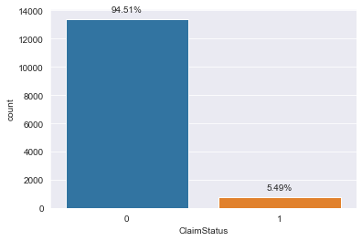
Figure 1: Count of Claim's status
The second dependent variable is the ClaimFrequncy and it gives the number of claims initiated by the policy holder. There are 5 unique values in this column ranging from 0 to 5. Its frequency is plotted in fig 2. From the plot it is evident that there is imbalances in the dataset, like in the case of claim status.
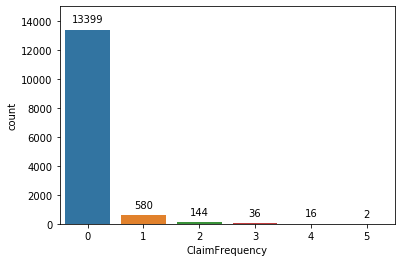
Figure 2: Count Plot of Claim Frequency
Now let’s investigate the relation between the ClaimFrequency and ClaimStatus. Since the two are categorical variable their count in relation to each other is tabulated in table 1. From the table it is evident that if claim frequency is greater than 0 then the claim status will be 1. There for we cannot use them as the independent variable for each other.
Table 1: Claim status vs Claim frequency
|
Claim Frequency |
||||||
|
Claim Status |
0 |
1 |
2 |
3 |
4 |
5 |
|
0 |
13313 |
0 |
0 |
0 |
0 |
0 |
|
1 |
0 |
575 |
137 |
34 |
16 |
2 |
Premium is our only continues variable which shows the amount in $1000 paid by the policy holder for the coverage. Fig 2 shows the boxplot of the distribution of the premium amount for each of the claim status. It shows that the customers who pays more than $250,000 as premium tends to initiate claim more often. Also there are 38 records that beyond the whisker of the largest boxplot, there for we treat them as outliers and removed from the dataset.
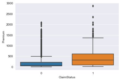
Figure 3: Boxplot of Claim status vs Premium
Billing Term represents how often the premium is paid. It is paid as once, thrice or six timesa year. The distribution of premium amount against the billing term is shown in fig 3.
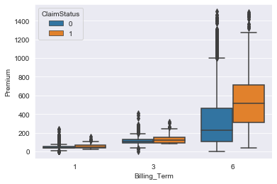
Figure 4: Boxplot of billing term vs Premium for each of the ClaimStatus
For billing terms of 1 and 2 the premium amount increases slightly but there no significant difference between then in terms of claims status. But when the billing term becomes 6 times a year the increase in premium amount is relatively higher.
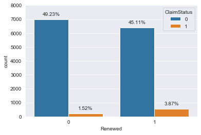
Figure 5: Count Plot of Renewed against the claim status
Fig 4 shows the count plot of the variable Renewed where 0 indicates the policy wasn’t renewed and 1 indicates otherwise. The figure shows a balanced distribution of the variable and it is evenly distributed across the claim status. Thus we can conclude that the variable Renewed doesn’t influence our target variable, ClaimStatus.
From the dataset we can remove the variables which contains the names of the excluded drivers since it doesn’t give any additional information about the claim status. Also in this dataset some variables are given as a set of five, this represents the data of the drivers listed in the policy. For each of the drivers these variables gives information on the date of birth, how long the driver has been driving, distance to work, marital status, occupation, relation to the main policy holder, gender and violation points.
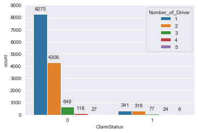
Figure 6: Number of drivers listed in the policy
The number of drivers listed in the policy grouped by the claim status is plotted in fig 5. For both the claim statuses, the number of records for more than 3 drivers are very few. As these can be considered as outliers we can remove the information about the 4th and the 5th drivers. Similar to this as when there are more than one driver listed in the policy, which is around 33% of the data, the rest of the 66% will have a lot of missing data. There is no perfect way to impute the missing data in these case as all of them are legitimate and not a mistake. In order to avoid this problem we only keep the data about the main policy driver and keep the variable Number_of_Driver in the dataset.
Table 2: Mean of age of main policy holder grouped by claim status
|
Claim Status |
Age |
|
0 |
50.77 |
|
1 |
51.44 |
The table 1 shows the mean age of the main policy holder grouped by the claim status. We can see that there is not much difference in the mean value of the age.
The Amendment column gives the number of times the policy was amended and it is plotted in fig 6. Since the number of amendments greater than zero is very few and spread across more categories we can combine them together as a single one. The tabulated value after combining them is shown in table 2.
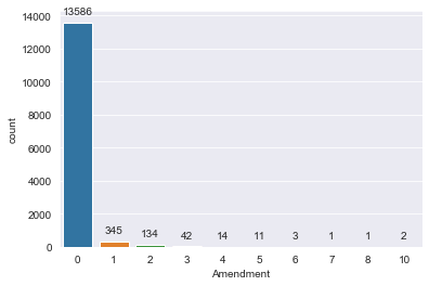
Figure 7: Count Plot of Amendments
Table 3: Number of amendments made on the policy
|
Amendments |
Count |
|
0 |
13,564 |
|
1 |
553 |
The violation points scored since second time is negligible in only one case does the total violation points for the entire data becomes larger than 10. So we only keep the information about the first violation points. The date of birth of each of the driver is converted to the age of the driver for making the analysis easier. The occupation details also has very high number of categories to have a meaningful insight there for we remove that information from dataset. The outliers and missing data in the year column is removed as it was very few. Similarly the column about the Make of the car is kept but Model of the car is removed. Since we have the total distance to work for all of the driver we can remove the columns that gives information about individual distance to work for each of the driver.
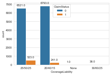
Figure 8: Count Plot of different coverage liability
In the CoverageLiability column three numbers are given for each records. They are the liability limit in thousands of dollars for per-person bodily injury, bodily injury for all persons injured in any one accident, and property damage liability respectively. Coverage liability represents the state's financial responsibility law i.e. the minimum requirement. The first figure is the amount to be paid for injuries per head, the second figure is the amount for all injuries and the third is the amount per vehicle damaged. In our dataset there are 3 types of such liability limits and for those records that doesn’t have it, “None” is used. Its distribution is shown in fig 7. Since the categories “None” and “30/60/25” has fewer values to make any meaningful result we eliminate those records from the dataset.
CoverageMP stands for Medical payments coverage. For an accident, this covers the medical expenses for the next three years. In the entire dataset only one record has positive value for this variable, there for we can eliminate this variable from the analysis. PD stands for Property Damage. This is a fundamental issue due to which every state makes it mandatory to have an auto insurance. It covers any damages to someone's property. The two figures in the column are the maximum coverage limit for a single property in an accident and all the properties in an accident respectively. Fig 8 shows the distribution of this variable.
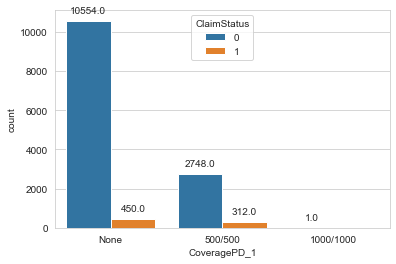
Figure 9: Count Plot of Coverage PD
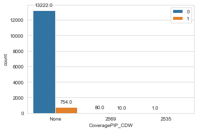
Figure 10: Count Plot of CoveragePIP_CDW
Since the category “1000/1000” has only one entry we can eliminate that record from ourdataset to simplify the analysis.
The count plot of the variable CoveragePIP_CDW is shown in fig 9. By applying the previous logic we can eliminate this variable also from the model. Similarly CoverageUMBI and CoverageUMPD has fewer number of records to have any meaningful impact on the model so we eliminate them also.
The Engine_1 column specifies the size of the engine in liters, the values greater that 15 are considered as outliers of this column and are replaced with the median of the values. The boxplot after managing the outliers is shown in fig 10.
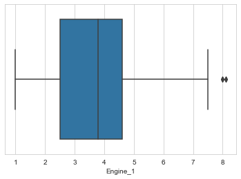
Figure 11: Boxplot of Engine size
The marital status and the sex of the main policy holder is plotted against the claim status in the figure 11.
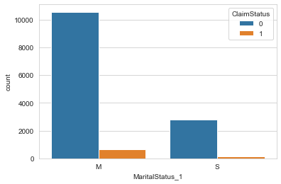
Figure 12: Marital status of the main policy holder
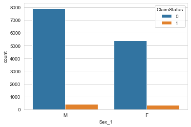
Figure 13: Gender of the main policy holder
The figure suggest that there might be a relation between the marital status and gender with the claim status.
The frequency of surcharge is plotted in fig 13. From this figure it is evident that only the third surcharge has any influence on the outcome, there for we keep the 3rd surcharge value and drop the other two.
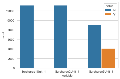
Figure 14: Count Plot of surcharge
Model
i) Claim Status
Since the data set we have is highly imbalanced with only 5.49% data represent one of two categories, we need to apply some techniques to remove the imbalance. In order to remove the imbalance in the data we’ve used up-sampling to improve the representation of the underrepresented category.
Then for the categorical variables, that are not already encoded numerically, we have used numerical labelling for encoding the data. For the numerical values normalization is done before feed it to the models as it would improve the efficiency of the classifier.
Then the data is split in to training data and test data in a ratio of 0.20. Then this training data is fed to different classification algorithms. The classification algorithms used for this purpose are Logistic regression, Random forest classifier, linear discriminant analysis, K-nearest neighbors, naïve Bayes classifier, and decision tree classifier and support vector machine.
ii) Claim Frequency
Here also the data is highly imbalance as shown in fig 2 and up-sampling is used to remove the imbalances. The same classification algorithms are used for easy comparison. The results are tabulated in table 4.
Table 4: Classification accuracy for different classifiers
|
Model |
Accuracy |
|
|
ClaimStatus |
ClaimFrequency |
|
|
Logistic Regression |
0.72 |
0.60 |
|
Random forest |
0.95 |
0.95 |
|
Linear discriminant analysis |
0.75 |
0.63 |
|
K-nearest neighbors |
0.86 |
0.85 |
|
Naïve Bayes Classifier |
0.77 |
0.15 |
|
Decision tree |
0.91 |
0.90 |
|
Support vector machine |
0.75 |
- |
Conclusion
The accuracies for different classification algorithms tried are tabulated in table 3. For both the dataset the highest accuracy is achieved for the ensemble methods, specifically Random forest. Random forest gave an accuracy of 95% in both cases. The worst performing model is the Naïve Bayes Classifier for predicting the Claim Frequency with an accuracy of 15% but it gave 77% accuracy for predicting Claim Status. Support vector machine didn’t run completely for predicting the Claim Frequency since it is a multi-class prediction and after the up-sampling for the 5 categories the number of rows were huge.
We can conclude from the above discussion on data analytics assignment that Random Forest is the best algorithm for our purpose. There is a high correlation between the premium amount and claim propensity of the existing customers. If the premium amount is low then the customer is more unlikely to claim than if the premium amount is high.


