Business Intelligence Assignment on Linear Programming & Transshipment

Question

Task

Prepare a detailed business intelligence assignment addressing the below questions:

Question 1 – Linear Programming and variants

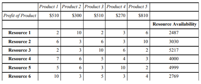
We wish to produce products - given constraints - so as to optimise our objective function. Bearing in mind the introductory material above, the questions follow below:

1a) Formulate a Linear Programming (an LP) model for this problem.

1c) Solve the problem - using Microsoft Excel Solver. Generate the Sensitivity report for the problem and name your Excel worksheet (spreadsheet tab) (e.g.) ‘Qu 1b Sensitivity Rep’.

1d) What is the optimal production plan (X1 , X2 , X3 , X4 , X5 ) and the associated profit? Refer to your answers to any of a), b) and/or c) above as appropriate.

For the remaining parts of this question, explain your answer(s), typically referring to relevant spreadsheet entry/ies and/or specific relevant parts of spreadsheet reports.

1e) Which constraints, if any, are binding? Refer to your answers to any of the above parts as appropriate, and explain your reasoning.

1f) The people running the company are now offered the opportunity of an exchange of goods.

The offer is for the company to receive 1 of Resource 2, 10 of Resource 4 and 100 of Resource 5 but for the company to have to relinquish (or surrender, or give away. or pay for these resources with) 10 of Resource 1, 5 of Resource 3 and 3 of Resource 6. Should the company accept this offer?

Clearly explain with clear calculations (to at least 3 decimal places) how much money the company would gain or lose by agreeing to such an exchange, making it clear whether this would result in a gain or a loss.

Let us return to the original problem above (prior to the company being made an offer) from part d. A proposal is put forward to produce a new product called Product 6.

Product 6 would have a profit of $155 and would require the following resources: 2 of Resource 2, 4 of Resource 4 and 5 of Resource 5.

1g) Would we expect Product 6 to be produced - i.e., if we are to produce products to optimise our objective function, would we produce any copies of this new product? If we would expect Product 6 to be produced, then how much less profitable could Product 6 be and still be produced?

If we would not expect Product 6 to be produced, then how much more profitable would Product 6 need to be in order to be produced?

Let us again return to the original problem above from part d, where the profitability of the various products was (510, 300, 510, 270, 810).

Various employees at the company have considered making changes which would affect the profitability of various products.

One change would result in (512, 301, 511, 269, 811)

1h) Explaining your reasoning, when compared to your original answer using (510, 300, 510, 270, 810), would your optimal amount to be produced of each of Product1, ..., Product5 change? Explain clearly why or why not. And, if the amounts produced would change, explain clearly with any necessary or relevant calculations what they would change to.

1i) A second change, if it really could be carried out in practice, would double the values to become (1020, 600, 1020, 540, 1620).

Explaining your reasoning, when compared to your original answer using (510, 300, 510, 270, 810), would your optimal amount to be produced of each of Product1, ..., Product5 change? Explain clearly why or why not. And, if the amounts produced would change, explain clearly with any necessary or relevant calculations what they would change to.

1j) A third change, which would probably not be a good idea, would halve the values to become (255, 150, 255, 135, 405).

Nonetheless, if such a change were to take place then, explaining your reasoning, when compared to your original answer using (510, 300, 510, 270, 810), would your optimal amount to be produced of each of Product1, ..., Product5 change? Explain clearly why or why not. And, if the amounts produced would change, explain clearly with any necessary or relevant calculations what they would change to.

1k) Returning to the original problem and solution from part d, suppose we now introduce the requirement that Product1, Product2 and Product 5 must be produced in equal amounts.

Compared to the original feasible region (from part d), does adding this new requirement make the feasible region larger, stay the same, smaller, or something else? Clearly explain your answer.

1l part 1) Continuing from part k with this newly introduced requirement that Product1, Product2 and Product 5 must be produced in equal amounts, what is the optimal amount to be produced of each of Product1, Product2, Product3, Product4, Product5?

11 part 2) What is the resultant profit (stated to at least 3 decimal places)? For both part 1 and part 2 of 1l, (in keeping with note 4,) clearly show all working.

Returning to the original problem from part d, suppose we now introduce the additional requirement that Product1, Product2, Product 3, Product 4 and Product 5 must be produced in integer amounts.

1m part 1) What is the optimal amount to be produced of each of Product1, Product2, Product3, Product4, Product5?

1m part 2) What is the optimal value of the objective function?

For both part 1 and part 2, (in keeping with note 4,) clearly show all working

1n) Continuing on from part m above, assume the same unit profits as before but now with fixed start-up costs as given below.

1n part 1) What is the optimal amount to be produced of each of Product1, Product2, Product3, Product4, Product5?

1n part 2) What is the optimal value of the objective function?

For both part 1 and part 2, (in keeping with note 4,) clearly show all working.

Question 2 – Transshipment and networks
Suppose we have a product (possibly masks, possibly shields, possibly containers of hand sanitiser) that we wish to move from two locations (let’s call them node 1 and node 2, both with a supply of 75) to two other locations (let’s call them node 7 and node 8, with demands of 80 and 70 respectively).

We initially assume the transportation costs along edges in the network to be as follows:

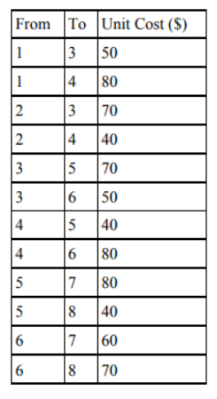
Students are expected and required to address question 2 in terms of linear programming (LP) and - if required - the closest possible variants.

2a) State the variables, and use these variables to state the objective function that we wish to optimise. (We assume that the cost is something that we wish to minimise.)

2b) How many variables are there? Informally in terms of the network, being as specific as you can, what do the variables correspond to?

2c) Solve the problem of the flow along edges giving the minimum cost. Show the amounts of flow along the edges. State the value of the objective function. State the number of edges with non-zero flow (and, for ease of reference, call this e2c ).

2d) Assuming that the number of edges with non-zero flow is less than e2c (equivalently, less than or equal to e2c - 1), again solve the problem of the flow along edges giving the minimum cost.

Show the amounts of flow along the edges. State the value of the objective function. State the number of edges with non-zero flow.

2e) If the problem is to have a solution of finite cost (any possible solution at all) in which goods get from the source/supply/starting points to the demand/sink destination points, what is the smallest number of edges that can have non-zero flow for such a solution to occur?

In that case (if we require that only this smallest possible number of edges be used), what is the minimum such cost? (If you followed the hint immediately above, then make sure to remove the newly introduced large penalty when giving your answer.)

2f) Return to the problem from parts a, b and c above.

Due to maintenance problems along the edge between node 4 and node 5, the unit cost of using this edge is $40/unit up to 30 units, then $60/unit thereafter.

Show how to solve this problem. In keeping with note 4, solve this problem.

2g) Following on from part f above, due to further maintenance problems along the edge between node 4 and node 5, the unit cost of using this edge is $40/unit up to 30 units, then $60/unit up to 55 units (i.e., we could have 30 units @ $40/unit and 25 units @ $60/unit, as 30 + 25 = 55), then $110/unit thereafter.

Show how to solve this problem. In keeping with note 4, solve this problem.

2h) We modify the original problem from parts a, b and c to be a shortest path problem. The edge costs (from parts a, b and c) should now be assumed to be the length of the edge. What is the shortest path from node 2 to node 8, and what is the length of the path?

Show how to solve this problem. In keeping with note 4, solve this problem.

2i part 1) Following on from part h, how would you modify your answer if we require that the path from node 2 to node 8 has to go through node 5?

2i part 2) Following on from part h, how would you modify your answer if we require that the path from node 2 to node 8 has to go through node 6?

Show how to solve this problem. In keeping with note 4, solve both parts of this problem.

Following on from the themes of part h and part i above, we now ask an open question worth bonus marks. (The motivation might be that someone has to collect face masks and shields on their way to a destination, but the order in which they collect them doesn’t matter.)

2j) Suppose we have a start node (call it A), and a destination node (call it D) and two intermediate nodes (call them B and C respectively) that we have to go through. Suppose also that we are allowed to go A to B to C to D and we are also allowed to go A to C to B to D, and that this is not known or specified in advance. How might we set this up as a linear programming (LP) problem?

We do not require a complete solution for 2j immediately above but wish you to explain in detail how you would set this up.

Answer

Answer 1 – Linear Programming and variants

1a) Formulation of a Linear Programming Model within this business intelligence assignment:
Given that there are 5 Different Products that are to be made with 6 Available Resources.

For Developing a LPP model,

Let’s assume,

Decision Variables

The Number of Units made of Product 1 be A

The Number of Units made of Product 2 be B

The Number of Units made of Product 3 be C

The Number of Units made of Product 4 be D

The Number of Units made of Product 5 be E

Given that the Profits of making Products 1,2,3,4,5 respectively are $510, $300, $510, $270, $810

Let’s assume the total profit is P

So,

Objective Function
P = (A*510) + (B*300) +(C*510) +(D*270) +(E*810)

Our aim should be to maximize the Profit, which is P.

The resource’s availability are Constraints.

Total Amount of Resource 1 required = 2A + 10B+ 2C+ 3D+ 6E

The maximum amount of resource A available = 2487

So,

2A + 10B+ 2C+ 3D+ 6E <= 2487

Similarly, for resource 2

6A + 3B+ 6C+ 3D+ 10E <= 3030

Similarly, for resource 3

2A + 3B+ 10C+ 6D+ 2E <= 5217

Similarly, for resource 4

7A + 6B+ 5C+ 4D+ 3E <= 4000

Similarly, for resource 5

5A + 6B+ 3C+ 10D+ 2E <= 4999

Similarly, for resource 6

10A + 3B+ 5C+ 3D+ 4E <= 2769

And also

Quantity of products can only be Non negative numbers

So,

A, B, C, D, E>= 0

1d)
Using Microsoft excel solver on the mathematical model, referring to row 8 of excel sheet “1b-LPP”

The optimal production plan to generate maximum profits is

Product 1: 4 Units with Profit of 4* 510 = 2040

Product 2: 83 Units with Profit of 83* 300 = 24900

Product 3: 277 Units with Profit of 277* 510 = 141270

Product 4: 365 Units with Profit of 365* 270 = 98550

Product 5: 0 Units with Profit of 0* 810 = 0

So, the optimal profit= 2040+ 24,900+ 141,270+ 98, 550+ 0= 266, 760

1e)
Here from the report from the solver in Microsoft Excel

“1b – LPP” Spreadsheet,

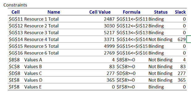
Resources 1,2,3,5 & 6 are completely utilized for making the prescribed quantities of Products in order to maximize the profits.

So, Constraint’s 1 ,2 ,3, 5, 6& 6 are binding

The same in shown in below report.

1f)
The offer for exchange is as follows,

The offer is for the company to receive 1 of Resource 2, 10 of Resource 4 and 100 of Resource 5 but for the company to have to relinquish (or surrender, or give away. or pay for these resources with) 10 of Resource 1, 5 of Resource 3 and 3 of Resource 6.

Making the changes according to the given exchange offer in the Mathematical model in spreadsheet “1f”

The new optimal solution is Producing a Profit of 266759.0323 which is less than the older profit of 266760.000

So, making this exchange would be losing an amount of $0.968

Hence making this exchange is not recommended.

1g)
From the results from solver in spreadsheet “1g”

We would not expect to produce Product 6 to maximize the Objective function.

From the sensitivity report in the spreadsheet “1g- Sensitivity”

For product 6 in order to be produced the profit should be at least 13.869 more than the original profit of 155.

1h)
Using (512, 301, 511, 269, 811) instead of (510, 300, 510, 270, 810) as the profits of the products.
From Sensitivity report in Spreadsheet “1b”

When we observe the allowable icrease and decrease from the sensitivity report above within this business intelligence assignment,

For Product A profits increase from 510 to 512 is not within the allowable increase of 1.333

For Product B profits increase from 300 to 301 is within the allowable increase of 22.5

For Product C profits increase from 510 to 511 is within the allowable increase of 8.780

For Product D profits decrease from 210 to 209 is within the allowable decrease of 5

For Product E profits increase from 810 to 811 is within the allowable increase of 48.339

Hence the Increase of Profit of Product A impacts the Optimal Solution.

1i)
If we make changes that would double the values to become (1020, 600, 1020, 540, 1620)

Since the values of all the coefficients of the Objective function is multiplied by 2, as given below, it doesn’t make any changes to the overall optimal amounts of each product to be produced.

P = { (A*510) + (B*300) +(C*510) +(D*270) +(E*810) } * 2

1j)
If we make changes that would halve the values to become (255, 150, 255, 135, 405).

Since the values of all the coefficients of the Objective function is divided by 2, as given below, it doesn’t make any changes to the overall optimal amounts of each product to be produced.

P = { (A*510) + (B*300) +(C*510) +(D*270) +(E*810) } * 1/2

1k)
Adding a constraint that the Product1, Product2 and Product 5 must be produced in equal amounts will make the feasible region smaller as the optimal solution has a extra constraint to deal with which are

A – B = 0

B – E = 0

1l part 1)
From spreadsheet “1k”

The optimal amount to be produced of each of Product1, Product2, Product3, Product4, Product5 are 9.685, 9.685, 271.384, 405.894, 9.685 respectively

1l part 2)
From spreadsheet “1k”

The optimal value of the objective function would be 263686.841

1m part 1)
If Product1, Product2, Product 3, Product 4 and Product 5 must be produced in integer amounts.

Adding this additional constraint in spreadsheet “1m”

The optimal amount ofProduct1, Product2, Product 3, Product 4 and Product 5 to be produced would be 4,83,277,365,0 respectively.

1m part 2)

The optimal value of the objective function is 266760.000

1n)
Now there is an extra constraint to deal with which is: in the sign restriction

A, B, C, D, E = Integers

And the objective function will change as,

P= (Total profit)- (Total fixed cost)

1n part 1)
From spreadsheet “1n”

The optimal amount to be produced of each of Product1, Product2, Product3, Product4, Product5 are 4, 83, 277, 365 and 0 respectively

1n part 2)
From spreadsheet “1n”

The optimal value of the objective function would be 235,760.000

1o)
Now there are two an additional constraint will be added to the model.

C>= 225 (The lower bound of the product 3)

C<= 325 (The upper bound of the product 3)

1o part 1)
From spreadsheet “1o”

The optimal amount to be produced of each of Product1, Product2, Product3, Product4, Product5 are 4, 83, 277, 365 and 0 respectively

1o part 2)
From spreadsheet “1o”

The optimal value of the objective function would be 235,760.000

1p)
Now there are three an additional constraint will be added to the model.

C>= 300 (The lower bound of the product 3)

C<= 450 (The upper bound of the product 3)

50C= integer

1p part 1)
From spreadsheet “1p”

The optimal amount to be produced of each of Product1, Product2, Product3, Product4, Product5 are 0, 93, 300, 317 and 0 respectively

1p part 2)
From spreadsheet “1p”

The optimal value of the objective function would be 235,490.000

1q)

1q part 1)
From spreadsheet “1q”

The optimal amount to be produced of each of Product1, Product2, Product3, Product4, Product5 are 4, 83, 277, 365 and 0 respectively

1q part 2)
From spreadsheet “1q”

The optimal value of the objective function would be 235,760.000

1r)

The new constraints

A= B (Product1 and Product2 are produced in equal abundance)

D= E (Product4 and Product5 are produced in equal abundance)

A+ B+ C= C (Product 3 is produced then neither product 1 nor product 2 is produced,)

E>= 10 (Product 3 is produced then at least 10 and at most 100 of Product 5 are produced.)

E<= 100 (Product 3 is produced then at least 10 and at most 100 of Product 5 are produced.)

1q part 1)
From spreadsheet “1r”

The optimal amount to be produced of each of Product1, Product2, Product3, Product4, Product5 are 0, 0, 483.333, 10 and 10 respectively

1q part 2)
From spreadsheet “1r”

The optimal value of the objective function would be 257, 300.000

Question 02

Network representation

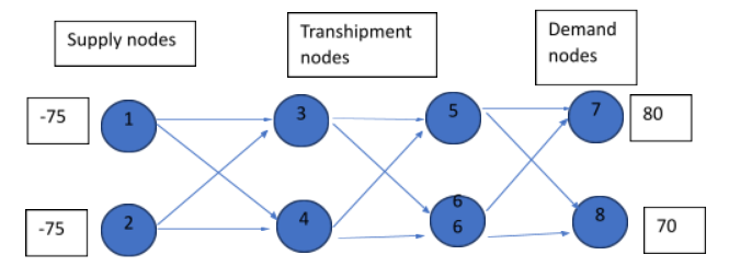
Total supply= -75- 75= -150

Total demand= 80+ 70= 150

So, the network is balanced. Then all the constraints have ‘=’ sign.

2a)
Variable declaration:

Let,

Xij = The number of products to be transformed from ith node to jth node.

Where,

I, j= 1, 2, 3, 4, 5, 6, 7, 8

Objective function

The objective function is to minimize the total transportation cost.

LP Model

Min z=50X13+80X14+ 70X23+40X24+ 70X35+50X36+40X45+ 80X46+80X57+ 40X58+60X67+ 70X68

S.T:

-X13-X14=-75 (At node 1)

-X23-X24=-75 (At node 2)

X13+X23-X35-X36=0 (At node 3)

X14+X24-X45-X46=0 (At node 4)

X35+X45-X57-X58=0 (At node 5)

X36+X46-X67-X68=0 (At node 6)

X57+X67=80 (At node 7)

X58+X68=70 (At node 8)

Xij ?0

2b)
Since there are 12 arcs in the network, there are 12 variables.

Each variable Xij corresponds to arc from node i to j

2c)
Amount flow along edges

Optimal cost= $21, 200

Number of edges with non-zero flow= 7

2d)
Amount flow along edges

Optimal cost= $24, 200

Number of edges with non-zero flow= 5

2e)
Let’s fix the cost values along below axis with big values (9999). Because these arcs have non-zero flows in the previous step.

X14, X24, X45, X57 and X58

Then the new optimal solution = $26,200

2f)
Using the senility report for the variables of the model, the allowable increase for X45 is 40. So, we can increase it until (40+40) =80 and 60 is within this range. So the allocation does not changed.

But optimal value will changed.

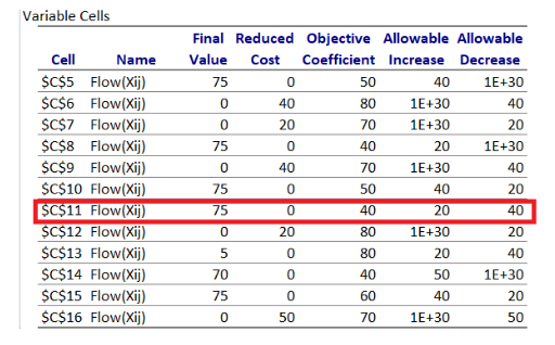
So the new objective value= (Previous value- (40*75)+(60*75))= 21, 200 + 1500= $22, 700

2g)
Using the senility report for the variables of the model, the allowable increase for X45 is 40. So, we can increase it until (40+40) =80.

But now 110 is out of the range. So, we need to resolve the model.

Then the optimal solution is:
Amount flow along edges

Optimal cost= $25, 500

2h)
New network representation for a shortest path problem from node 2 to node 8

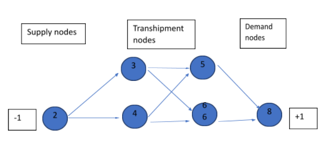
So, the new model is:

Variable declaration:

Let,

Xij ={1 ;If the path i?j is used tothe shortest path. 0 ;If the path i?j is not used tothe shortest path.

Where,

I, j= 2, 3, 4, 5, 6, 8

Objective function
The objective function is to minimize the total transportation cost.

LP Model
Min z= 70X23+40X24+ 70X35+50X36+40X45+ 80X46+ 40X58+ 70X68

S.T:

-X23-X24=-1 (At node 2)

X13+X23-X35-X36=0 (At node 3)

X14+X24-X45-X46=0 (At node 4)

X35+X45-X57-X58=0 (At node 5)

X36+X46-X67-X68=0 (At node 6)

X58+X68=1 (At node 8)

Xij =Binary

So, the shortest path is:

2-> 4-> 5-> 8

Length of the shortest path: 120

2i)
Part 1

With adding a new constraint s.t:

X35+X45=1 (At node 5 the new constraint)

So, the shortest path is:

2-> 4-> 5-> 8

Length of the shortest path: 120

Part 2

With adding a new constraint s.t:

X36+X46=1 (At node 6 the new constraint)

So, the shortest path is:

2-> 3-> 6-> 8

Length of the shortest path: 190