If you are a student pursuing your higher academic career in the discipline of mathematics or statistics, you would come to know that the frequency table entails a lot of significance on the stream of mastering the subject. To understand the major concepts in the theories related to statistics it becomes very urgent to learn the concept of frequency distribution table.

Definition of Frequency Distribution Table
A customized type of table which is majorly used to record down the value of some observation and its frequency of occurrence is termed to be a frequency distribution table. The frequency distribution table is widely used to arrange a huge set of data systematically in a corporate environment. This tool has the efficiency to simplify any complex data which is in the format of assigned value and frequency of its occurrence. In a generic form of frequency distribution table, customarily two columns are provided. Among these columns, the first one is assigned to record the value of a particular variable, and the second one is assigned to record the frequency of the occurrence of the relevant variable at a certain point. If the complex data is arranged according to this table, then it would get very easy to handle the whole data. The different columns in the frequency table could be tagged as column A and Column B. As mentioned above in this report, the frequency should be noted down in column B.

Relevant Implication of Frequency Distribution Table
To get an understanding of the core concept of the frequency distribution table in a thorough manner, you should consider an example. This would make you acquainted with the methodology and calculations in the frequency distribution table. Let us consider the below example provided in this report.

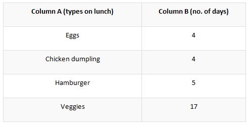
Take an instance, that a certain person is having veggies as his food. In the calendar month, the person had eaten the veggie diets on 1^st, 2^nd, 4^th, 6^th, 7^th, 8^th, 11^th, 13^th, 14^th, 17^th, 19^th, 20^th, 22^th, 25^th, 27^th, 29^th, 30^th as the mid-day meal. As a cheat from the followed diet, the person had eaten hamburger on the date of 3^rd, 9^th, 12^th, 16^th, 23^rd in the same month. He had also followed the intermittent diet of eggs on the dates of 21^st, 24^th, 26^th, 28^th and the chicken dumplings on the dates of 5^th, 10^th, 15^th, 18^th in the same year. By keeping in mind, the afore given data, you could prepare a frequency distribution table as provided in the below format.

By using the frequency distribution table provided above, it could be analyzed that, how strictly the person had followed the veggie diet. It could be noted that the person had followed the diet very frivolously since he had eaten the veggie-only for 17 days in the bracket of a month.

Distinct varieties of frequency distribution table
The frequency distribution could be classified into five types as mentioned in the discipline of statistics. They could be listed as: –

• Relative frequency distribution
• Ungrouped frequency distribution
• Relative cumulative frequency distribution
• Grouped frequency distribution
• Cumulative frequency distribution

Different types of customized tables should be used in different types of frequency distribution mentioned in the above section. Let us discuss the variations and the mode of implications followed in each type of frequency distribution table.

Grouped and Ungrouped Data
A set of figures or pieces of information which is logged over a period of time is signified by the term data. In data, various components could be included which may be numerical figures, units, or string of words. The knowledge of both grouped and ungrouped sets of data would be very important since without the knowledge of it the frequency distribution table could not be executed accurately.

Ungrouped data
In the discipline of statistics, the ungrouped data could also be termed as raw data. This is been called so because there is no categorization in data and is presented in a very scattered manner. The data in the group would be so random that the categorization is not much convenient. Let us take an example of the data collected from the census. The data would be very large and considering them under a particular category would be very hard. The ungrouped form of data is generally used to represent some random data collected from a large population. The major benefit of using the ungrouped data is that the comprised pieces of information that could be interpreted and calculated very effortlessly. Since it is very simple to handle this type of data set the calculator doesn’t need to possess any technical knowledge. The calculation is considered to be easy since the data could only be segregated into smaller groups, and statistical ratios like skewness, mean, mode, median, etc. could be estimated without any effort.

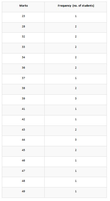
Let us assume an example of the ungrouped set of data on which the ungrouped frequency distribution is being applied for the estimation of ratio. In this section, we have taken the context of 30 students who have attended the test for English. It should be taken into account that the exam was taken from a total of 50 marks. The marks obtained by the 30 students are 49, 43, 28, 36, 42, 32, 39, 33, 44, 45, 43, 32, 39, 41, 38, 44, 37, 33, 38, 46, 44, 45, 34, 39, 23, 36, 47, 48, 34, 28.

Below is given the frequency distribution table applied to this groupset.

Grouped data
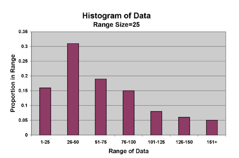
If a collected piece of data is being segregated into different sections then it would get qualified to be called as grouped data. Various sections in the data would be dealing with different variables and hence assigning them to different groups becomes very necessary to do. Hence while carrying out the calculation with a group data the initial format of raw information is transformed into one which consists of various and columns tagged under the denomination of various variables. Since there are many variables comprised in this form of data, the final calculation could be done by following various methodologies. The most common and popular form of classification in this division is classifying the observations under different classes by which segregation is done according to the magnitude of each observation. Let us take an example of marks scored by different students in a class. You could create different classes for the marks obtained by the students in the class. Let us take an instance that a student had scored 93 out of 100, you could include the observation of that person under the class of 90 – 100. In the case of grouped data, the classification and the calculations could be best displayed using the tool of histograms or frequency distribution table. Below is provided an example of a histogram that is drawn from the instance of observation collected from the marks scored by different students in a certain class.

By using the grouped set of data, the power to approximate a certain statistical mean point increase. The estimating ability increases because the person could emit the observation or population which is irrelevant for the calculation. In the grouped system of data, the segregation of the data could be done in a very balanced manner.

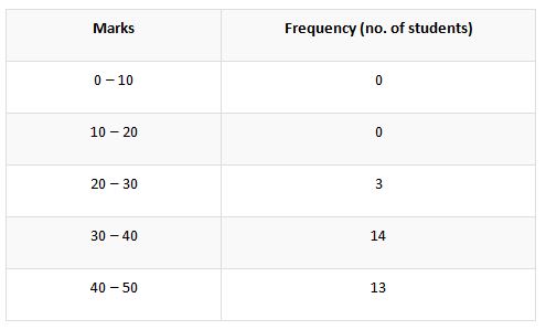
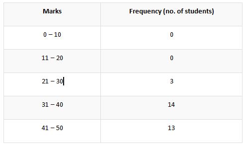
The instance of marks obtained by 30 students as mentioned in the above case under the ungrouped data. Now we are going to segregate the earlier data by the method of grouped frequency distribution table. Let us look at the below table.

The column tagged with the word, marks denotes the classes by why which the marks are classified. In the distribution of the classifying classes, there is both a lower limit and a higher limit. For elucidation let us take the class interval of 30 – 40. In this class, the higher limit could be perceived as 40 and the lower limit as 30.

This approach towards the group of data is a very exclusive one. The limits mentioned in the segregation could comprise of all the observations provided. This means if an interval like 0 – 10 is taken, all the observations having the numerical value in between 0 a 10 are comprised in it.

Although this segregation is not much complicated, most of the students find it difficult to handle the data in the grouped frequency table format. Because of this reason, most of the time the estimation of statistical data is done very inaccurately in this method. Hence to reduce the complication in the approach a more inclusive is taken to handle the ungrouped frequency distribution table. And hence as a consequence of it, the intervals between the classes are changed.

In the below table the same data set is taken like that in the above section of this report. Let us have a better look at this inclusive format of data.

You could observe of the manipulations done in the first column of marks or the segregation of classes. It is being done to simplify the situation like the occurrence of the value like 40, 30, 10, 30, etc. If the class is being manipulated like this the values with 0 at one’s digit place could be allotted easily to the customized classes.

Here it could be understood that the grouped frequency distribution table uses two columns which should be customized as per the gaps in between the classes. There should be continuity between the assigned classes so that there should be no complication to assign any of the observations into it.

Cumulative Frequency Distribution table
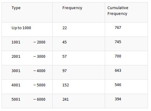
Among all the methods used in data handling, the cumulative frequency distribution is undisputedly the most efficient and relevant one. The efficient and exclusive use of cumulative format is done in the recording process of frequency in the table. Let us get into the methodology to calculate and handle the data using the approach of the cumulative frequency distribution table.

• You could use the approach of adding up the frequencies as you gradually move downwards in the frequency distribution table. In each step, the frequencies are summed up with the cumulative amount.
• It is based upon the frequency observed in each class that the gradual accession of cumulative frequency is calculated. The cumulative frequency calculated in the previous or upper column is being added with the present frequency.

For a better understanding of the methodologies to be followed in the calculation of the cumulative frequency table, an example is provided below. Let us have a detailed look at it.

Relative frequency distribution table
By using the tool of the relative frequency distribution table, the number of occurrences or the recognition of a certain article could be ascertained in a very accurate and effort-free manner. In this process, a certain sample is selected from the population and based on this sample the trend is calculated. The major trend is estimated by observing the frequency of a certain incidence and is a very effective tool in the corporate world. The relative frequency distribution is signified in the terms of percentage, not in the nominal integer denominations.

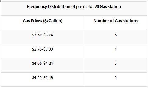
Below is provided an effective way of using the relative frequency on a certain date. You should learn and understand the methodology to be followed in this section since it has great practicability in the real world.

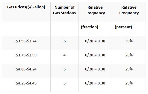
In this method, the calculation is not limited to a single table, and the next format displays the prices in the layout of relative frequency. The effective changes in the reflective frequency taking the basis of the individual class is displayed below.

In this case, the resultant value of the relative frequency is being divided by the denomination of 20, which is equivalent to the number of gas stations. Unlike the other methods, mentioned, the values in this method are either represented in the form of a fraction or percentage. By using the tool of the frequency distribution table, the efficient comparison between two entirely different data sets could be conducted.

Relative cumulative frequency distribution
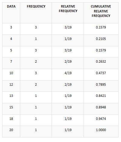
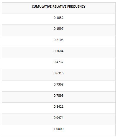
In this approach, the cumulative frequency is being divided by the aggregate frequency, and hence the relative cumulative frequency could be obtained. Let us take a data set which comprises of 19 entries that specified the usual distance covered by the individuals to reach their workplace. Below is given the set of observations.

10; 18; 5; 12; 13; 12; 4; 5; 10; 2; 5; 7; 3; 2; 10; 18; 15; 20; 7;

The frequency distribution regarding the given set of data could be arranged as per the table provided in the below section.

It could be quite evident that you get suspicious of whether the provided calculation or the format provided above is correct or not. The way to find any abnormality would not be too difficult in this approach. Don’t panic, the above-given format is accurate. Although you could check it by adding the frequency. The overall sum should add up to 19, and if not, then the illustration is wrong.

Below is provided the cumulative relative frequency, please have a thorough look at it.

We hope that you have now attained all the knowledge about the frequency distribution table. Let us now look at the detailed aspect of the evolution of the frequency distribution table. For a student pursuing his degrees in statistics or other related subjects, the concept of frequency distribution sale bears the highest significance. If you find it very hard or demanding, the assignments for statistics you could also approach us for a quality solution. Let us have a look at the frequently asked question by our students regarding the frequency distribution table.

FAQ

What is it meant by frequency distribution?

The depiction of the provided set of data in the form of either graph or any specified tabular format exactly provides the occurrences of a particular value or incidence in the provided span of period. The major significance of the distribution majorly lies in determining the trend and simplification of the calculation in calculating the statistical ratios. By using the table which is customized for displaying the frequency distribution, the overall distribution of the values could be determined. As per the parameter of distinct classes and the related frequencies of the observations the overall data provided in the set is arranged and segregated.

What are the three different variants of the frequency distribution?

Cumulative frequency distribution, grouped frequency distribution, and ungrouped frequency distribution comprise all the three-chief sort of frequency distributions. If the selected set of variables could be classified into various categories the whole set could be termed as a grouped set. The selected set of values that satisfies the parameter of possessing an interval width of a single unit could be termed as ungrouped frequency distribution. For convenience, the components in the ungrouped set are arranged in the ascending manner of their numerical value. In the discipline of statistics, the most popular form of the frequency distribution is the cumulative form of frequency distribution table. In this stage, the frequency values are added to each step of the class intervals. Hence automatically being arranged in the ascending order.